How To Model The Coronavirus Part 1
- Joel Runevic

- May 8, 2020
- 9 min read
Introduction
Hello and welcome to another post! This is the beginning of a series of posts on how to model the Coronavirus outbreak! No matter where you are in the world, you must have heard of the Coronavirus (formally known as COVID-19) pandemic. It has spread all around the world, reaching 3.5 million cases. Unfortunately, over a quarter of a million people have died due to this virus, as of 5th May 2020. Many countries, as a result, have been put into a strict lockdown to try and prevent the virus from spreading.
This post is designed to help you develop your own model of the Coronavirus outbreak. Keep in mind that this is a relatively simple model and is mainly designed to help you better understand what is currently going on in the world. Moreover, I hope that it will help you to better appreciate why many countries have entered a 'lockdown' and the drastic consequences that would have happened if this was not the case. In order to make your own, you can simply use Google Sheets (which is free!) or Microsoft Excel, if you have purchased the software package. Without further ado, let's begin!
R0-Value
If you have kept up with the news, you may be familiar with the idea that the value of R0 has to be less than one. I mean here in England, where I am from, the government is constantly talking about how the value of R has to be less than one, or, as Prime Minister Boris Jonhson put it; "driving down the R" is the country's "collective endeavour." But what is R?
In epidemiology (the branch of medicine that essentially studies how diseases spread), the value of 'R0' basically describes the average number of people an individual can expect to infect. The reason why the 'R value' is so important is because it dictates the spread of the virus and its overall impact on a country and the world as a whole. If the value of R is greater than one, the virus will spread exponentially.
For example, let's suppose that the value of R was 2 for COVID-19 and I was the only person infected with the virus. Mathematically speaking, I will infect 2 other people with the virus. Those two individuals will then infect 2 more people each. As a result, excluding myself and the two people that I infected, there will now be four more infected individuals. These four individuals will then infect two more people each and the process will continue, with the number of infections increasing exponentially. This is bad - really bad - and soon, if no measures were put in place to bring the value of 'R' down, healthcare systems around the world could have been overwhelmed with critical COVID-19 cases. This is essentially why governments imposed a strict lockdown - to bring the value of R down.
Now that you understand more about the vital 'R value', we can begin looking at the other variables that are important, when it comes to modelling the Coronavirus outbreak.
The Variables
We are going to be creating a simple epidemic model called the SIRD model. We are going to split the entire population (the entire population of England, in this case) into four different categories: susceptibles, infected, recovered, and dead.
Susceptibles refer to the individuals who are capable of being infected with COVID-19; we will assume that this is the entire population of England (which is 56 million, as of 2020); I have decided to use the population of England, and not the UK, as England's lockdown rules may differ from Wales' or Scotland's et cetera. The category 'infected' refers to the individuals who have COVID-19 and therefore can spread it to other individuals. The 'recovered' variable states how many individuals have recovered from COVID-19 and are therefore assumed to be no longer infectious. This model assumes that once an individual has recovered from COVID-19 they can longer become infected in the future - in other words, they will always stay 'Recovered'. The other, final, variable, 'Dead', refers to the number of individuals who have unfortunately died from the Coronavirus, once they have been infected with it. In other words, an individual in the 'Susceptibles' state can either stay in this state or transition into the 'infected' state. Once 'infected', an individual can then either become 'Recovered' or, due to the virus, transition into the 'Dead' state.
You may have an idea of what the initial value will be for each variable; however, we are going to decide on the value for each respective category once we actually begin creating the model itself. For now, we are just focusing on the theory behind the model.
The Equations
For this model to successfully operate, we are going to use a system of differential equations. That sounds very complicated and, in reality, it is. However, we do not need to concern ourselves about solving the system of equations, but, rather, we are more interested in analysing the results that come from the said system of equations. In other words, we are going to be looking at the rate of change with respect to time of each of our variables.
Firstly, we must begin to understand what the derivative of each variable really means and can begin with dS/dt. This is the derivative of S with respect to t (where t represents the time passed in days and S is the number of susceptibles). In our context, this refers to how the number of susceptible people is changing in time. We can apply the same reasoning to the other derivatives (dI/dt, dR/dt, and dD/dt). The derivative of each variable is simply stating how the number of susceptible, infected, recovered or dead invidiuals is changing with respect to time.
Now that we understand what each derivative is telling us, we can begin to actually form the system of equations, beginning with dS/dt. If we think about it logically, the only way for a susceptible individual to be infected by COVID-19 is that they come into close proximity with an infected individual. Once this happens, there is a probability that the susceptible person will then become infected themselves. In other words, the more connections there are between infected, I, individuals and susceptible, S, individuals, the greater the increase in infections will be, resulting in an increased rate of change for S with respect to time.
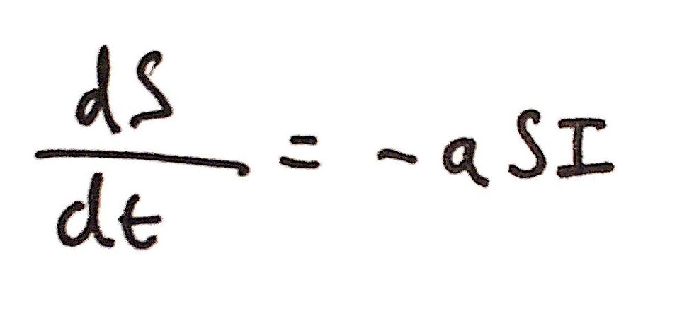
We can thus argue that the value of dS/dt is proportional to the two variables, S and I, multiplied by each other. We will also multiply SI by -a, where 'a' denotes the infection rate (more on this later) - remember, just because an infected person meets a susceptible person does not mean that the susceptible person will certainly get infected and thus we have the constant of proportionality 'a'. The negative also denotes that the number of total Susceptibles is decreasing as more and more individuals are infected. I have included an image of the differential equation for dS/dt below:
Now we can turn our attention to dI/dt. In order for there to be an increase in the number of infected individuals, there must be a corresponding decrease in the number of susceptibles. From our differential equation above, we can therefore see that this increase in infected people is equivalent to aSI (note: there is no negative as the number of infected individuals is increasing). However, there are two other factors that affect the number of infected individuals. These two factors are 'bI' (where b is just a constant of proportionality or the 'recovery rate') and 'cI' (where c is just another constant of proportionality or the 'death rate'). These factors must be subtracted from aSI as they represent infected individuals who transition into either a recovered state or a dead state. The final differential equation for dI/dt is as follows:

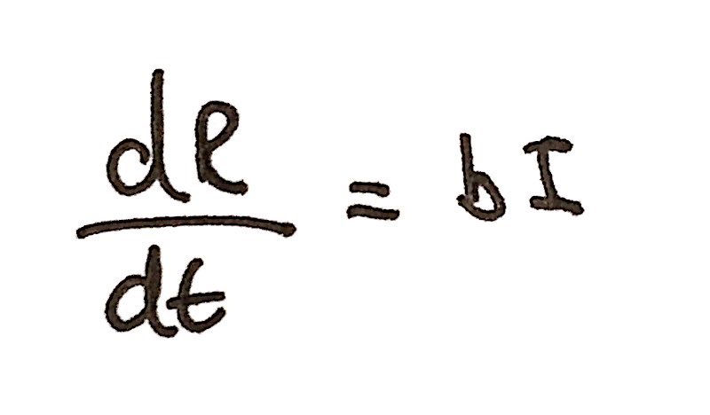
The differential equation for dR/dt is just bI. This represents the proportion of infected individuals who have successfully recovered from COVID-19. The rate at which this happens is dependent on the recovery rate 'b'. In our model, we will take the value of b (which we will calculate later) to be an average for our entire population; in other words, it does not vary due to an individual's age or other factors. For a clearer image of the value for dR/dt, see below:
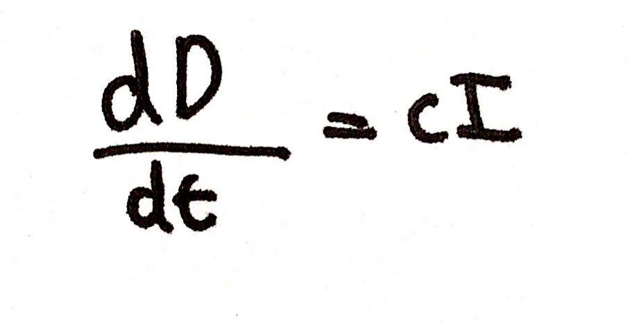
We can apply the same principle to dD/dt. This is simply cI as it depends on the number of infected individuals and the death rate, 'c'. Note that all the constants (a, b, and c) are all taken to be positive. I have included an image of the differential equation for dD/dt below:
Thus, we get our system of differential equations. All four of these equations must be true at the same time. Like I said before, we are not concerned about how to solve this system of equations; we are instead interested on the quantitative data that we can extract from this system of equations. We can now dive deeper into what our system of differential equations really means, and we can now incorporate that all-important 'R value' we talked about before.
Where Does The 'R' Value Fit Into All Of This?
If we focus on the differential equation for dI/dt, we can begin to understand where the 'R0' value can be incorporated. After all, the number of infected people pretty much dictates the course of an epidemic. The initial number of infected individuals can be labelled as 'I0' and the initial number of Susceptibles can be labelled as 'S0'. If we look at dI/dt and consider the value of dI/dt at time t=0, so, in other words, when the epidemic just begins, the key condition is whether dI/dt is less than 0. If it is below 0, then there may be new cases of infected individuals, but the rate of increase in said infected cases is slowing down and thus the number of infected individuals will eventually reach 0. In other words, people will die or recover from COVID-19 quicker than new individuals can get infected from the virus, resulting in the disease eventually dying out. However, if it is above 0, then the rate of infected individuals will be increasing, resulting in exponential growth, and the epidemic will be very much alive. In effect, the statement shown in the image below is what we are considering (note: you can just divide by I0 on both sides to simplify):

From here we can just rearrange the equation, in a few steps, to get the equation below:

We can now just represent the left-hand side of the condition (with all the constants) as our 'R0' as I have included below:

This, therefore, allows us to analyse how the values of a, b, c, and S0 impact the value of 'R' (which we already know from before is responsible for how large a disease epidemic becomes). From just analysing the type of relationship between each variable and R, we can see how governments and individuals can lower the value of R. For example, if 'a', which can be viewed as the transmission rate, was lowered, due to more individuals washing their hands, that would also lower the value of R. Moreover, if the value of S0, the number of people initially susceptible, was lower, due to say a large proportion of the population being vaccinated, so will the value of R be lowered. This is due to the fact that both a and S0 are directly proportional to the value of R.
On the other hand, both the constants b and c (representing the recovery rate and death rate, respectively) are inversely proportional to the 'R' value. For example, if new drugs that assist the immune system against COVID-19 were to be discovered, the value of b will increase (as a greater proportion of individuals will recover from the disease) and thus the value of R will decrease as they are inversely proportional.
What is quite interesting is the impact of the death rate, 'c', on the R value. Having a greater death rate, 'c', means that the value of R will be lower. This is due to the fact that if individuals die at a greater rate then they will be less able to infect other individuals, which is partly why very deadly diseases do not tend to lead to global pandemics in modern times. However, of course, we don't want this death rate to be high and thus governments try to reduce the value of 'R' by decreasing the value of a and S0 or, on the other hand, by increasing the value of b. This is why the government has imposed the lockdown and is looking so desperately for a vaccine against the virus - in order to "drive down the R". The lower the R, the lower the rate of transmission of the virus, and the quicker the epidemic will end, which is why it is so important to abide by lockdown rules and to always wash your hands!
Although we will calculate the different constants (a, b and c to name a few) using a different method for our model in Part 2, I believe that it is very important to understand in what context the 'R0' value will fit into our model, what impact it has and how the value of 'R' can be changed by governments and individuals alike.
That is it for Part 1! We have now successfully determined what our main variables will be and have developed a system of differential equations, which will prove very useful later. Also, we have now understood where the 'R' value comes from, and the impact it has on the transmission of a virus. Stay tuned for Part 2, where we will begin developing our model using Google Sheets / Microsoft Excel. Thank you very much for you time. Feel free to comment any questions you may have and please share this article with your friends!


Comments