Finding the Shortest Path
- Sriram A

- Aug 29, 2020
- 7 min read
Pathfinding is one of the most essential concepts in computing today. It is used in many complex tasks, from the programming of an enemy AI which follows the player in a landscape filled with obstacles to finding the best roads to drive through to reach the destination in the shortest time on Google Maps.
Many algorithms exist for this task. But almost all of them are heavily based on Djikstra's algorithm, so we will explore this one first. Please note that I have adapted the original algorithm slightly for a grid-based version, as I have used final distances instead of unvisited sets. In this implementation, I will be using a priority queue optimization.
Dijkstra's Shortest Path Steps:
Mark all nodes unvisited.
Initialize an empty priority queue.
Assign a tentative distance to every node: zero for the starting node and infinity for all the other nodes.
Mark the starting node as the current node.
Set the tentative distance of the current node as its final distance.
For each unvisited node surrounding the current node:
Calculate a new tentative distance (current node final value + distance between adjacent node and current node)
If the newly calculated tentative distance is lower than the node's current assigned value then replace the adjacent node's tentative distance with the newly calculated tentative distance, and push the adjacent node's tentative distance and a reference to the node as a key-value pair to the priority queue.
6. Mark the current node as visited.
7. If the end node has been visited, the algorithm has finished. If not, proceed to step 8.
8. Pull the next current node from the priority queue (node with the lowest tentative distance) and repeat from step 5.
As I coded this algorithm using Python, I used the built-in Priority Queue module. This implementation of the priority queue makes use of a binary heap, so we can take the find-min operation to have a time complexity of O(1) and the decrease-key operation to have a time complexity of O(log(n)).
This means the overall complexity of this implementation of Dijkstra's Shortest Path will be O(log(E) + V), where E is the number of edges and V is the number of vertices. This algorithm is admissible; it will always return an optimal solution. This can be proven by induction on the number of nodes visited.
This implementation can certainly be optimized and I would encourage you to look at ways you can optimize it after reading this article; I will provide the source code at the end.
Here's a visualization of Dijkstra's shortest path algorithm with no obstacles:
The red square is the start node, and the green square is the end node. The blue nodes represent visited nodes, and the cyan nodes represent explored nodes (unvisited nodes with a non-infinite working value). The shortest path is drawn at the end in yellow.
As you can probably tell, the main disadvantage of this algorithm is that it performs a blind search when finding the shortest path. Although this guarantees an optimal solution, it is relatively time-consuming. It can also only be used on a weighted graph with positive weights.
Here are some more visualizations, which include obstacles:

An easy way to build upon and improve this algorithm is by adding an additional function estimating the distance between a node and the end node. This is known as a heuristic, and it is how the A-Star algorithm build's on Dijkstra's.
A Star Algorithm Steps:
Mark all nodes unvisited.
Initialize empty priority queue.
Assign a G Cost to every node. This will be set to infinity for all nodes except from the starting node.
Mark the starting node as the current node, and set its G Cost to 0.
For each unvisited node surrounding the current node:
Calculate a new G Cost (current node G Cost + distance between adjacent node and current node)
If the newly calculated G Cost is lower than the node's current assigned G Cost then replace the adjacent node's tentative distance with the newly calculated G Cost.
Calculate a H Cost for the node: a heuristic estimate of the distance between the node and the end node.
Calculate the F Cost by adding the G Cost and H Cost together.
Push the adjacent node's reference and its F Cost to the Priority Queue
Mark the current node as visited.
7. If the end node has been visited, the algorithm has finished. If not, proceed to step 8.
8. Pull the next current node from the priority queue (node with the lowest F Cost) and repeat from step 5.
The worst case time-complexity of the A-Star Pathfinding Algorithm is O(log(E) + V), which is the same as Dijkstra (if the H Cost was completely wrong every time). But in most situations the A Star Algorithm will perform faster than Dijkstra's, depending on what heuristic is used for the H Cost.
Here's a visualization of the A-Star Pathfinding Algorithm:
There are many different heuristic functions one can use with this algorithm, and demonstrating these is much easier when there are obstacles present.
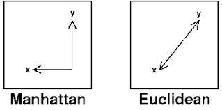
Here is one visualization using a Euclidean distance heuristic:
Here is one with similar obstacles, but with a Manhattan distance heuristic instead:
The Euclidean distance heuristic is the "straight-line distance" between two points, i.e. as the crow flies. The Manhattan distance heuristic takes the absolute values of the difference in x and y coordinates of two points and adds them together.
We can also add these two together to create a new heuristic function as shown below:
There are a variety of different heuristic functions one can use, and deciding which is most suitable will depend on the situation in which the algorithm is being applied. This is also a disadvantage of the A-Star Algorithm: its admissibility is dependent on the heuristic function. This means the A-Star algorithm may not always return the shortest path.
Below is the code used to make the visualization of the A-Star Algorithm. You can run this to create your own obstacles and experiment using different heuristics. Creating the Dijkstra Algorithm from this should not be too difficult. My code can certainly be optimized and I would encourage you to try this. I hope you enjoyed reading this post!
import numpy as np
import pygame
import queue

pygame.init()
size = width, height = 300, 300
block_width = 10    # setting rendered block size
nodeWidth, nodeHeight = int(width/block_width), int(height/block_width)   # setting node grid size
screen = pygame.display.set_mode(size)
clock = pygame.time.Clock()
grid = []
pq = queue.PriorityQueue()
pq2 = queue.PriorityQueue()


class NODE:
    def __init__(self, position):
        self.position = position
        self.walkable = True
        self.visited = False
        self.g_cost = 100000
        self.h_cost = 0
        self.f_cost = 100000
        self.on_path = False
        self.previous = None
        self.explored = False

    def __lt__(self, other):
        return self.f_cost < other.f_cost


def precision_number(n):
    return round(n, 5)


def unit(n):
    if n > 0:
        return -1
    else:
        return 1


def render():   # render function; in hindsight I should've added a colour property to the Node class
    for i in range(nodeWidth):
        for j in range(nodeHeight):
            if grid[i][j] == start_node:
                pygame.draw.rect(screen, (255, 0, 0), [grid[i][j].position[0] * block_width,
                                                       grid[i][j].position[1] * block_width,
                                                       block_width, block_width])
            elif grid[i][j] == end_node:
                pygame.draw.rect(screen, (0, 255, 0), [grid[i][j].position[0] * block_width,
                                                       grid[i][j].position[1] * block_width,
                                                       block_width, block_width])
            elif not grid[i][j].walkable:
                pygame.draw.rect(screen, (0, 0, 0), [grid[i][j].position[0] * block_width,
                                                     grid[i][j].position[1] * block_width,
                                                     block_width, block_width])
            elif grid[i][j].on_path:
                pygame.draw.rect(screen, (255, 255, 0), [grid[i][j].position[0] * block_width,
                                                         grid[i][j].position[1] * block_width,
                                                         block_width, block_width])
            elif grid[i][j].visited:
                pygame.draw.rect(screen, (0, 0, 255), [grid[i][j].position[0] * block_width,
                                                       grid[i][j].position[1] * block_width,
                                                       block_width, block_width])
            elif grid[i][j].explored:
                pygame.draw.rect(screen, (0, 255, 255), [grid[i][j].position[0] * block_width,
                                                         grid[i][j].position[1] * block_width,
                                                         block_width, block_width])
            else:
                pygame.draw.rect(screen, (255, 255, 255),
                                 [grid[i][j].position[0] * block_width, grid[i][j].position[1] * block_width,
                                  block_width, block_width])
    pygame.display.flip()


for i in range(nodeWidth):  # initializing the node grid
    grid.append([])
    for j in range(nodeHeight):
        node = NODE(np.array([i, j]))  # each node is created with an index referencing its position on the grid
        grid[i].append(node)
grid = np.array(grid)
# start node
start_node = grid[1][1]  # set this to whatever you want within the range of the node grid
start_node.g_cost = 0
start_node.visited = True
# end node
end_node = grid[28][28]  # set this to whatever you want within the range of the node grid
end_node.on_path = True
pq.put((0, start_node))
previous_node = None

drawing = False
erasing = False
start = False

while not start:  # drag your mouse across the window to draw and press enter to start the algorithm
    render()
    for event in pygame.event.get():
        if event.type == pygame.KEYDOWN:
            if event.key == pygame.K_LSHIFT:
                erasing = True
            if event.key == pygame.K_RETURN:
                start = True
        elif event.type == pygame.KEYUP:
            if event.key == pygame.K_LSHIFT:
                erasing = False
        if event.type == pygame.MOUSEBUTTONDOWN:
            drawing = True
        elif event.type == pygame.MOUSEBUTTONUP:
            drawing = False
        if event.type == pygame.MOUSEMOTION and drawing:
            if erasing:
                pos = pygame.mouse.get_pos()
                pos = tuple(map(lambda x: int(x / block_width), pos))
                grid[pos].walkable = True
            else:
                pos = pygame.mouse.get_pos()
                pos = tuple(map(lambda x: int(x / block_width), pos))
                grid[pos].walkable = False

# look at all nodes adjacent to current node
# for each node, calculate the f cost
# f cost = g cost + h cost
# g cost = cost of node from start node
# h cost = heuristic estimate of cost of node to end node
# mark current node as explored
# choose the node with the lowest f cost to explore next

while not end_node.visited:
    pygame.event.get()
    current_node = pq.get()[1]
    current_node.previous = previous_node
    render()

    for i in grid[current_node.position[0]-1: current_node.position[0]+2]:
        for j in i[current_node.position[1]-1: current_node.position[1]+2]:
            vector = j.position - current_node.position
            try:
                if not j.visited and j != current_node and j.walkable \
                        and not (not grid[j.position[0] + unit(vector[0])][j.position[1]].walkable  # handling diagonals
                                 and not grid[j.position[0]][j.position[1] + unit(vector[1])].walkable):
                    cost_from_current = np.linalg.norm(current_node.position - j.position)
                    cost_to_end = sum(list(map(lambda x: abs(x), end_node.position - j.position)))  # Manhattan Distance
                    cost_to_end += np.linalg.norm(end_node.position - j.position)   # Euclidean Distance
                    if j.g_cost > cost_from_current + current_node.g_cost:
                        j.g_cost = cost_from_current + current_node.g_cost
                    j.h_cost = cost_to_end
                    if j.f_cost > j.h_cost + j.g_cost:
                        j.f_cost = j.g_cost + j.h_cost
                        j.explored = True
                        pq.put((j.f_cost, j))
            except IndexError:  # used when the search area exceeds the dimensions of the grid
                pass
    current_node.visited = True
    previous_node = current_node

current_node = end_node

while not start_node.on_path:  # tracing the path
    current_node.on_path = True
    pygame.event.get()
    for i in grid[current_node.position[0] - 1: current_node.position[0] + 2]:
        for j in i[current_node.position[1] - 1: current_node.position[1] + 2]:
            if j != current_node and not j.on_path:
                pq2.put((j.g_cost, j))
    current_node = pq2.get()[1]
    render()

while 1:
    for event in pygame.event.get():
        if event.type == pygame.QUIT:
            pygame.quit()


Comments