Teaching an AI to play video games

Landing an aeroplane; performing a complicated surgery; fighting a case in court. These are jobs that normally require humans to undergo many hours of intense training, and even after that, something goes wrong. But what if a computer could do that job? Would it be better or worse for humanity if we passed these high intensity jobs to AI? These exciting ideas may soon become reality with the help of rapid developments happening in machine learning, particularly within reinforcement learning.

Fundamentally, almost every reinforcement learning technique is implemented in an environment framework known as a Markov decision process. This is a common framework used for optimization problems such as the one we are exploring today.

The key decision maker within this framework is known as the agent, and it can observe and interact with its environment, known as the observation space. This is sort of analogous to a player within a video game.

A Markov decision process can be represented by the following tuple:

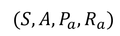
S represents the set of states the agent can be in, known as the state space.

A represents the set of actions the agent can take from the set of states S.

Pa(S, S’) represents the probability that an action a in state sat time t will result in state s’ at time t + 1.

Ra(S, S’) is the expected immediate reward when the agent transitions from state s to s’ after taking the action a.

The goal of reinforcement learning is to maximize the cumulative reward for an agent interacting with its environment. This is done by selecting an action a from state s such that the reward Ra(S, S’) plus the sum of all rewards from future steps taken from the state s’ is maximised.

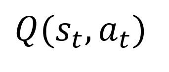
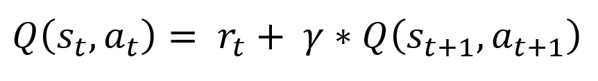
The algorithm we will use to find and optimize Ra(S, S’) is known as Q-Learning. Within this algorithm, the reward r given from taking an action a in a state s at time t is known as a Q-Value. This can be denoted as the Q function:

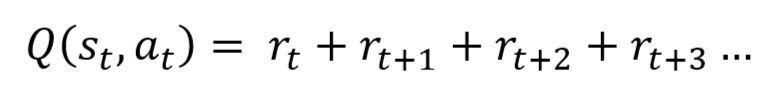
As stated before, the Q value of a state action pair can be given as the sum of the immediate reward plus the total of all future rewards of actions succeeding the action taken from the state:

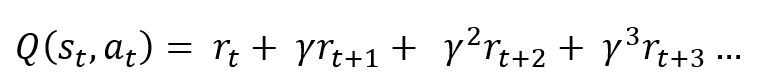
However, at time t, we are only given the information, and cannot be completely certain about the reward given from future actions, so a discount rate must be applied at each time step after the current state:

But how would we go about calculating all these future rewards and discounting them? This can be done by looking at the expression for the Q-Value of the state succeeding the current one:

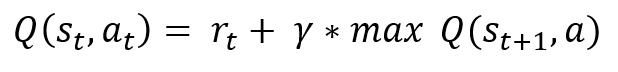
This expression is already present in Q(s,a) for the current time step, so we can simplify it:

It can also be assumed that an action a taken from any state s is taken such that the Q-Value of the state Q(s ,a) is the maximum available Q-Value from the current state. Thus the expression can be simplified further:

This is the optimal Q-Value function approximation. During our training process we push our values towards this value at a certain learning rate alpha:

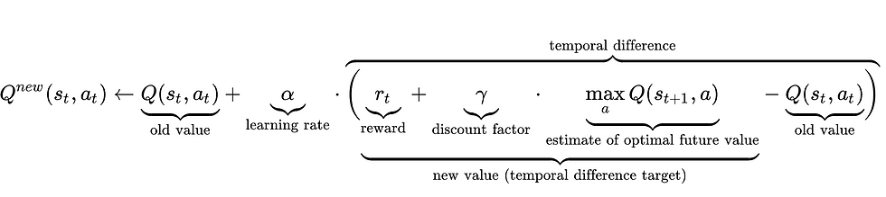
Credits to wikipedia.org

An array of all of the possible discrete state action pairs is stored, known as the Q-Table, and every time an agent performs an action and enters a certain state the Q-Value for that state action pair is updated using the formula shown above.

With the maths out of the way, we can start coding. To implement this algorithm we will use the Mountain Car environment from Open-AI gym, which comes with plenty of support for multiple machine learning algorithms.

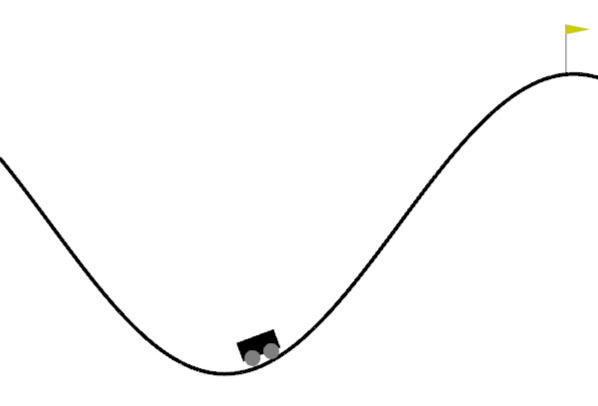
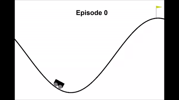
Our agent is the car, and its goal is to reach the flag on top of the hill.

If you do not already have the following libraries, please install them:

pip install gym

pip install matplotlib

Before we set up the environment, we must make our Q-Learning Agent. Start by importing numpy into a new python file:

import numpy as np

We will use numpy to create our array of Q-Values. For our Q-Learning Agent to be recognized as an object, we must create a class for it, along with an initialization function. The first parameters we require as arguments are the dimensions of our environment's observation space.

class QLearningAgent:
    def __init__(self, env):
        self.high = env.observation_space.high.astype('float64')
        self.low = env.observation_space.low.astype('float64')

This returns the maximum and minimum values in the MountainCar observation space. Because Q-Learning requires a discrete observation space, we have to split the continuous observation space up into bins so we can create a Q-Table with a fixed size. We can then use the array of maximum (or minimum) values to create a set of bins. Each continuous observation value will fall within one of these discrete bins.

class QLearningAgent:
    def __init__(self, env, bin_number):
        self.high = env.observation_space.high.astype('float64')
        self.low = env.observation_space.low.astype('float64')
        self.bin_number = bin_number
        self.os_width = self.high - self.low
        self.discrete_bin_number = [bin_number] * len(self.high)

We can now create our Q-Table with random values initially. It has the dimensions discrete state * action space. This allows us to simply input the state our agent is in and get the action required as an index of the action containing the maximum Q-Value for that state.

class QLearningAgent:
    def __init__(self, env, bin_number):
        self.high = env.observation_space.high.astype('float64')
        self.low = env.observation_space.low.astype('float64')
        self.bin_number = bin_number
        self.os_width = self.high - self.low
        self.discrete_bin_number = [bin_number] * len(self.high)        
        self.q_table = np.random.uniform(0, 1, self.discrete_bin_number + [env.action_space.n])

And the final parameters we must add are the discount factor, learning_rate and the number of discrete actions we can take. When the agent takes an action, we pass the action as a number between 0 and the number of actions we can take to the agent.

class QLearningAgent:
    def __init__(self, env, bin_number, discount_factor, learning_rate, *args, **kwargs):
        self.high = env.observation_space.high.astype('float64')
        self.low = env.observation_space.low.astype('float64')
        self.bin_number = bin_number
        self.os_width = self.high - self.low
        self.discrete_bin_number = [bin_number] * len(self.high)
        self.q_table = np.random.uniform(0, 1, self.discrete_bin_number + [env.action_space.n])
        self.discount_factor = discount_factor
        self.learning_rate = learning_rate
        self.action_number = env.action_space.n

Next we need to define a function which converts continuous states to discrete states. From our agent we recieve an array containing the information required. If we convert this array to a decimal value between 1 and 0, 1 being the maximum values of the observation space and 0 being the minimum, we can multiply it by the number of bins per value in the state, and convert this to an integer value. This returns a discrete state.

def get_state_as_discrete(self, state):
    state = state.astype('float64')
    state = tuple((((state - self.low) / self.os_width * self.bin_number).astype('int')))
    return state

Now we need to define a function which selects an action based on our Q-Table array. We do this by receiving the state the agent is in, and using the np.argmax() function. The argmax function returns the index number of the maximum value in the given list. In this case it is an integer between 0 and 1 (drive left or right).

def select_action(self, state):
    action = np.argmax(self.q_table[state])
    return action

Now we need a function that actually carries out the Q-Learning algorithm. This function will be called every step and takes the old state, new state, the action taken and the numerical reward received from taking this action. It then carries out the Q-Value update by referring to the appropriate values as explained previously. Over time the Q-Values will update to an optimal state which gives the highest cumulative reward.

def update_q_values(self, state, new_state, action, reward, *args, **kwargs):
    old_q = self.q_table[state + (action, )]
    optimal_future_q = np.max(self.q_table[new_state])
    new_q = old_q + self.learning_rate * (reward + self.discount_factor * optimal_future_q - old_q)
    self.q_table[state + (action, )] = new_q

Now we can implement our Q-Agent in the environment. Before we do this you can run the following code in a new python file to make sure your gym module is working properly:

import gym
env = gym.envs.make('MountainCar-v0')
env.reset()
while True:
    env.step(0)
    env.step(1)
    env.render()

env.reset() resets the car position. env.step() passes the action to the agent. In this case there are two actions: driver right and drive left. env.render() renders the update in an animation in a separate window.

Start by creating a new python file and importing gym and the python file we created our agent in. I named my file "q_agent.py"

import gym
import q_agent

We can now create our environment and create our Q-Learning Agent. The values selected for the parameters, apart from 'env', can be anything as long as they are of the correct data type. I would encourage anyone following along to experiment with these and see how results vary.

env = gym.envs.make('MountainCar-v0')
agent = q_agent.QLearningAgent(env=env, bin_number=20, discount_factor=0.95, learning_rate=0.2)

Now we need to declare the number of episodes our Q-Learning agent will run for. Each episode will last until the car reaches the flag or it runs out of time.

EPISODES = 10000
for episode in range(EPISODES):

At the start of each episode, we need to reset the agent's position in the environment so that the car starts at the bottom of the hill. This can be done using env.reset(), which also functions to provide us with the starting state of our agent. We also need to create a variable representing whether the episode is done or not, and set this to False at the start of each episode.

for episode in range(EPISODES):
    Done = False
    env.reset()
    state = agent.get_state_as_discrete(env.reset())

Within this for loop we can now create a while loop which runs once each episode. The following steps occur:

1. An action is selected based on the state the agent is in, using the function we created previously.

2. The agent executes the action, and we receive back information about the new state the agent is in, the reward the agent received from executing the action in the previous state and whether the episode is done.

3. We then convert our new state to a discrete state.

4. Using all of this information, we can update the q-values in our q-table by passing the appropriate arguments

while not Done:
    env.render()
    action = agent.select_action(state)
    new_state, reward, Done, _ = env.step(action)
    new_discrete_state = agent.get_state_as_discrete(new_state)
    agent.update_q_values(state=state, new_state=new_discrete_state, action=action, reward=reward)
    state = new_discrete_state

This is pretty much all we need for our Q-Learning agent to run and learn. However, this algorithm would take a very long time to learn if we rendered every single episode, so we can put in an additional piece of code so that only every 100th episode is rendered.

while not Done:
    if episode % 100 == 0:
        env.render()
    action = agent.select_action(state)
    new_state, reward, Done, _ = env.step(action)
    new_discrete_state = agent.get_state_as_discrete(new_state)
    agent.update_q_values(state=state, new_state=new_discrete_state, action=action, reward=reward)
    state = new_discrete_state

This was the result after training for 600 episodes.

Code so far:

Q-Learning Agent:

import numpy as np


class QLearningAgent:
    def __init__(self, env, bin_number, discount_factor, learning_rate, *args, **kwargs):
        self.high = env.observation_space.high.astype('float64')
        self.low = env.observation_space.low.astype('float64')
        self.bin_number = bin_number
        self.os_width = self.high - self.low
        self.discrete_bin_number = [bin_number] * len(self.high)
        self.q_table = np.random.uniform(0, 1, self.discrete_bin_number + [env.action_space.n])
        self.discount_factor = discount_factor
        self.learning_rate = learning_rate
        self.action_number = env.action_space.n

    def get_state_as_discrete(self, state):
        state = state.astype('float64')
        state = tuple((((state - self.low) / self.os_width * self.bin_number).astype('int')))
        return state

    def update_q_values(self, state, new_state, action, reward, *args, **kwargs):
        old_q = self.q_table[state + (action, )]
        optimal_future_q = np.max(self.q_table[new_state])
        new_q = old_q + self.learning_rate * (reward + self.discount_factor * optimal_future_q - old_q)
        self.q_table[state + (action, )] = new_q

    def select_action(self, state):
        if np.random.random() < self.epsilon:
            action = np.random.randint(0, self.action_number - 1)
        else:
            action = np.argmax(self.q_table[state])
        return action
        

Q-Learning Process:

import gym
import q_agent

env = gym.envs.make('MountainCar-v0')
agent = q_agent.QLearningAgent(env=env, bin_number=20, discount_factor=0.95, learning_rate=0.2)
EPISODES = 1000

for episode in range(EPISODES):
    Done = False
    env.reset()
    state = agent.get_state_as_discrete(env.reset())
    episode_reward = 0
    while not Done:
        if episode % 100 == 0:
            env.render()
        action = agent.select_action(state)
        new_state, reward, Done, _ = env.step(action)
        new_discrete_state = agent.get_state_as_discrete(new_state)
        agent.update_q_values(state=state, new_state=new_discrete_state, action=action, reward=reward)
        state = new_discrete_state
env.close()

As you could probably tell, the method the car uses to finally reach the flag is far from an optimal one. In my next post I will cover techniques we can use to improve its efficiency. Thank you for reading this post!